P&S Module 2018

In this session, we focus on introducing basic concepts and techniques in Digital Image Processing and Computer Vision. We also would like to discuss how you can apply these techniques to Machine Learning tasks. Note that we omit many mathematical details that are out of the scope of the session.

Digital Image Representation

Before giving intuitive examples of digital images or simply images, we would like to formally define the concept of digital image and digital image processing. One accurate definition is from the book Digital Image Processing (2nd Edition) by Rafael C. Gonzalez and Richard E. Woods.

An image may be defined as a two-dimensional function, $f(x,y)$ , where $x$ and $y$ are spatial (plane) coordinates, and the amplitude of $f$ at any pair of coordinates $(x,y)$ is called the intensity or gray level of the image at that point. When $x$ , $y$ , and the amplitude values of $f$ are all finite, discrete quantities, we call the image a digital image. The field of digital image processing refers to processing digital images by means of a digital computer.

Remark: Although this book was published over a decade ago, the book presents a comprehensive introduction that both beginners and experts can enjoy reading.

With the above definition, we can define an image as a $n\times m\times k$ (height x width x color_channels) array where the image consists of $n\times m$ pixels and $n, m, k\in \mathbb{N}^{+}$ . The resolution of an image is also determined by the number of pixels of the image.

A pixel is a point $(x,y)$ in an image. Typically, the intensity of a pixel is denoted as one or an array of uint8 values. uint8 is unsigned 8-bit integer that has the range $[0, 255]$ (0 is no color, 255 is full color). If there is only one color channel ( $k=1$ ), the image is typically stored as a grayscale image. The intensity of a pixel is then represented by one uint8 value where 0 is black and 255 is white. If there are three color channels ( $k=3$ ), we define that the first, the second and the third channel are the red channel, the green channel and the blue channel respectively. We hence refer this type of image to as RGB color image. The intensity of a pixel in a RGB image is represented by three uint8 integers where these three integers express the mixture of the three base colors - red, green and blue. You can interpret the value of a certain channel as the degree of the color intensity. Because each pixel has three uint8 values, each RGB pixel can represent $2^{24}$ different colors.

The grayscale and the RGB encodings are only two types of image color-spaces. There are other image color-spaces such as YCrCb, HSV, HLS that are widely applied in many other applications. We do not discuss these color-spaces here.

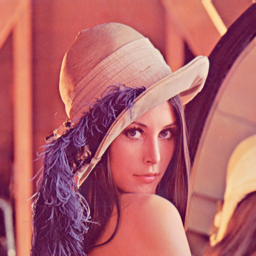
Lenna: Goddess of Digital Image Processing.

The above picture is one of the most famous testing images - Lenna (or Lena). The resolution of the image is $512\times 512$ . The image has both simple and complex textures, a wide range of colors, nice mixture of detail, shading which do a great job of testing various of image processing algorithms. Lenna is truly goddess of digital image processing. If you would like to read more story of Lenna, please follow this link.

Given a grayscale or RGB image, we can naturally treat the image as the same as a matrix or a 3D tensor. We can then process images with our knowledge of Linear Algebra.

Image Geometric Transformation

This section introduces some simple ways for manipulating images such as scaling, translation, rotation and affine transformation. These geometric transformations are presented with the help of OpenCV and scikit-image.

OpenCV is an optimized Computer Vision library that supports multiple programming languages. The library implements many classical and modern Image Processing and Computer Vision related algorithms very efficiently. In this module, we use the Python bindings of the OpenCV. If you have installed the OpenCV, you can import the package in your program as follows:

import cv2

scikit-image (or skimage) is an optimized image processing library that belongs to the scikit-learn family of libraries. This library focuses on supporting image processing functions that are important to Machine Learning tasks. To import this package in your program:

import skimage

Scaling

Scaling (resizing) an image concerns with the topic of up-sampling and down-sampling. For example, the Max-Pooling operation we introduced in Session 3 is a way of scaling an image. In this section, we shell use the OpenCV’s API to rescale an image.

import cv2
import numpy as np

# read the image file
img = cv2.imread("Lenna.png")  # put the lenna.png at the same directory as the script

# fx: scaling factor for width (x-axis)
# fy: scaling factor for height (y-axis)
res = cv2.resize(img, None, fx=2, fy=2, interpolation=cv2.INTER_CUBIC)

#OR

# extract height and width of the image
height, width = img.shape[:2]
# resize the image
res = cv2.resize(img, (2*width, 2*height), interpolation=cv2.INTER_CUBIC)

# display the image
cv2.imshow('rescaled', res)
cv2.waitKey(0)
cv2.destroyAllWindows()

Yo can find the detailed documentation of the cv2.resize from here

Note that OpenCV reverse the color channel order while encoding an RGB image. OpenCV refers this encoding to as BGR. OpenCV uses the BGR as the default color space. However, if you would like to process and plot the RGB image using other libraries, you will need to convert the channel ordering via the cvtColor API:

res_rgb = cv2.cvtColor(res, cv2.COLOR_BGR2RGB)

For skimage, one can achieve the same effect via imread and resize APIs:

from skimage.io import imread
from skimage.transform import resize
from skimage.transform import rescale

import matplotlib.pyplot as plt

# read the image file
img = imread("Lenna.png")

# resize the image
height, width = img.shape[:2]
res = resize(img, (height*2, width*2))

# OR
# rescale the image by factor
res = rescale(img, (2, 2))

# display the image
plt.figure()
plt.imshow(res)
plt.show()

Check out the detailed documentation at here.

Translation

Image translation shifts the content of an image to another pre-defined location.

import cv2
import numpy as np

# read the image, 0 means loading the image as a grayscale image
img = cv2.imread("Lenna.png", 0)
rows,cols = img.shape

# define translation matrix
# move 100 pixels on x-axis
# move 50 pixels on y-axis
M = np.float32([[1, 0, 100],[0, 1, 50]])
# translate the image
dst = cv2.warpAffine(img, M, (cols, rows))

# display the image
cv2.imshow('img', dst)
cv2.waitKey(0)
cv2.destroyAllWindows()

In the above example, one has to define a translation matrix M:

$M = \left[\begin{matrix} 1 & 0 & 100 \\ 0 & 1 & 50 \end{matrix}\right]$

Essentially, the above translation matrix shifts the pixel at $(x, y)$ to the new coordinations $(\hat{x}, \hat{y})$ :

$\begin{aligned} \hat{x}&=x+100 \\ \hat{y}&=y+50 \end{aligned}$

In skimage, one can translate the image by using the warp and SimilarityTransform APIs:

from skimage.io import imread
from skimage.transform import warp
from skimage.transform import SimilarityTransform

import matplotlib.pyplot as plt

# read image
img = imread("Lenna.png", as_grey=True)

# translate the image
tform = SimilarityTransform(translation=(-50, -100))
warped = warp(img, tform)

# display the image
plt.figure()
plt.imshow(warped, cmap="gray")
plt.show()

Rotation

Rotation of an image for an angle $\theta$ in OpenCV is achieved by defining a rotation matrix that has the form of

$M = \left[\begin{matrix} \cos\theta & -\sin\theta \\ \sin\theta & \cos\theta \end{matrix}\right]$

You can compute this matrix in OpenCV via the getRotationMatix2D API. The following example rotates the image for $45^{\circ}$ in counter-clockwise direction.

import cv2

# read the image in grayscale
img = cv2.imread("Lenna.png", 0)
rows, cols = img.shape

# rotate for 45 degree counter-clockwise respect to the center of the image
M = cv2.getRotationMatrix2D((cols/2, rows/2), 45, 1)
dst = cv2.warpAffine(img, M, (cols, rows))

# display the image
cv2.imshow('img', dst)
cv2.waitKey(0)
cv2.destroyAllWindows()

In skimage, one can perform this operation via rotate API:

from skimage.io import imread
from skimage.transform import rotate

import matplotlib.pyplot as plt

# read image
img = imread("Lenna.png", as_grey=True)

# rotate the image for 45 degree
dst = rotate(img, 45)

# display the rotated image
plt.figure()
plt.imshow(dst, cmap="gray")
plt.show()

Affine transformation

Affine transformation is a linear mapping method that preserves points, straight lines and planes. In affine transformation, all parallel lines in the original image will still beg parallel in the output image.

In the following example, we select three points from the original image (in this case, $x_{1}=(50, 50)$ , $x_{2}=(200, 50)$ , $x_{3}=(50, 200)$ ). They will be mapped to the new coordinations $\hat{x}_{1}=(10, 100)$ , $\hat{x}_{2}=(200, 50)$ , $\hat{x}_{3}=(100, 250)$ .

import cv2
import numpy as np
import matplotlib.pyplot as plt

# read the image
img = cv2.imread("Lenna.png", 0)
rows, cols = img.shape

# select three points
pts1 = np.float32([[50, 50], [200, 50], [50, 200]])
pts2 = np.float32([[10, 100], [200, 50], [100, 250]])

# get transformation matrix
M = cv2.getAffineTransform(pts1, pts2)

# apply Affine transformation
dst = cv2.warpAffine(img, M, (cols, rows))

# display the output
plt.subplot(121), plt.imshow(img, cmap="gray"), plt.title('Input')
plt.subplot(122), plt.imshow(dst, cmap="gray"), plt.title('Output')
plt.show()

The corresponding skimage version of the affine transformation is as follows:

import numpy as np 
from skimage.io import imread
from skimage.transform import warp
from skimage.transform import estimate_transform

import matplotlib.pyplot as plt

# read image
img = imread("Lenna.png", as_grey=True)

# define corresponding points
pts1 = np.float32([[50, 50], [200, 50], [50, 200]])
pts2 = np.float32([[10, 100], [200, 50], [100, 250]])

# estimate transform matrix
tform = estimate_transform("affine", pts1, pts2)
# apply affine transformation
dst = warp(img, tform.inverse)

# display the output
plt.subplot(121), plt.imshow(img, cmap="gray"), plt.title('Input')
plt.subplot(122), plt.imshow(dst, cmap="gray"), plt.title('Output')
plt.show()

Note that the above code estimates the transformation matrix using estimate_transform API. If there is a predefined linear mapping, one can also specify the transformation matrix using the AffineTransform API.

Simple Image Processing Techniques

Image thresholding

Thresholding may be one of the most straightforward Computer Vision algorithms. Given a grayscale image, each pixel is assigned to a new value that depends on the original pixel intensity and a threshold.

Why is the thresholding useful? For example, if the image texture is simple enough, one can carefully design a threshold so that the desired portion of the image can be selected. In other cases, if you would like to investigate the illumination level of the image, you can also apply thresholding to do it.

If you apply a global threshold to the entire image, it may not be good in all the conditions because different regions of the image have different lighting conditions. In this case, we can consider adaptive thresholding methods. For example, we first calculate the threshold for a small regions of the image. And then use the calculated value on local region to threshold pixels.

import cv2
import numpy as np
from matplotlib import pyplot as plt

# load the image
img = cv2.imread("Lenna.png", 0)

# apply global thresholding
ret, th1 = cv2.threshold(img, 127, 255, cv2.THRESH_BINARY)

# apply mean thresholding
# the function calculates the mean of a 11x11 neighborhood area for each pixel
# and subtract 2 from the mean
th2 = cv2.adaptiveThreshold(
    img, 255, cv2.ADAPTIVE_THRESH_MEAN_C,
    cv2.THRESH_BINARY, 11, 2)

# apply Gaussian thresholding
# the function calculates a weights sum by using a 11x11 Gaussian window
# and subtract 2 from the weighted sum.
th3 = cv2.adaptiveThreshold(
    img, 255, cv2.ADAPTIVE_THRESH_GAUSSIAN_C,
    cv2.THRESH_BINARY, 11, 2)

# display the processed images
titles = ['Original Image', 'Global Thresholding (v = 127)',
          'Adaptive Mean Thresholding', 'Adaptive Gaussian Thresholding']
images = [img, th1, th2, th3]

for i in xrange(4):
    plt.subplot(2, 2, i+1), plt.imshow(images[i], 'gray')
    plt.title(titles[i])
    plt.xticks([]), plt.yticks([])
plt.show()

A skimage implementation of global thresholding and adaptive thresholding is:

from skimage.io import imread
from skimage.filters import threshold_adaptive

import matplotlib.pyplot as plt

# read image, note that pixel values of the image are rescaled in the range of [0, 1]
img = imread("Lenna.png", as_grey=True)

# global thresholding
th1 = img > 0.5

# mean thresholding
th2 = img > threshold_adaptive(img, 11, method="mean", offset=2/255.)

# gaussian thresholding
th3 = img > threshold_adaptive(img, 11, method="gaussian", offset=2/255.)

# display results
titles = ['Original Image', 'Global Thresholding (v = 127)',
          'Adaptive Mean Thresholding', 'Adaptive Gaussian Thresholding']
images = [img, th1, th2, th3]

for i in xrange(4):
    plt.subplot(2, 2, i+1), plt.imshow(images[i], 'gray')
    plt.title(titles[i])
    plt.xticks([]), plt.yticks([])
plt.show()

Filtering

In last session, we discussed how a filter in ConvNet can be used to produce feature map. The process of applying a filter is convolution. This is also at the core of implementing static convolution filters. You can in principal design a filter that is sensitive to certain spatial patten. In result, you can obtain the interesting signal.

Here we demonstrate how can you use an average filter to blur an image.

The average filter that has $M\times N$ elements is defined as follows:

$M=\frac{1}{MN}\left[\begin{matrix} 1_{11} & 1_{12} & \cdots & 1_{1N} \\ 1_{21} & 1_{22} & \cdots & 1_{2N} \\ \vdots & \vdots & \ddots & \vdots \\ 1_{M1} & 1_{M2} & \cdots & 1_{MN} \end{matrix}\right]$

The average filter, as the name suggested, computes the average value over the filtered region. If we apply this filter on every possible region, then the image will be blurred because each pixel now is a mixture of multiple pixels in a local region.

import cv2
import numpy as np
from matplotlib import pyplot as plt

# read the image
img = cv2.imread("Lenna.png")

# prepare a 11x11 averaging filter
kernel = np.ones((11, 11), np.float32)/121
dst = cv2.filter2D(img, -1, kernel)

# change image from BGR space to RGB space
img = cv2.cvtColor(img, cv2.COLOR_BGR2RGB)
dst = cv2.cvtColor(dst, cv2.COLOR_BGR2RGB)

# display the result
plt.subplot(121), plt.imshow(img), plt.title('Original')
plt.xticks([]), plt.yticks([])
plt.subplot(122), plt.imshow(dst), plt.title('Averaging')
plt.xticks([]), plt.yticks([])
plt.show()

Remark: Unfortunately, there is no obvious implementation for skimage in this case. But this can be achieved by using other numerical packages such as scipy to perform this task.

Gradients, again

In some cases, spatial changes on the image may be attractive to know. For example, if someone want to find the shape of an object in the image, we usually assume that the region round the edge of the object will change dramatically. With this spatial change, we can then define the spatial gradient.

Here we demonstrate two kinds of gradient filters: Laplacian filters and Sobel filters. Here we demonstrate some common settings of these two filters

Laplacian filter:
$M=\left[\begin{matrix} 0 & 1 & 0 \\ 1 & -4 & 1 \\ 0 & 1 & 0 \end{matrix}\right]$
Sobel filter for horizontal edge:
$M=\left[\begin{matrix} 1 & 2 & 1 \\ 0 & 0 & 0 \\ -1 & -2 & -1 \end{matrix}\right]$
Sobel filter for vertical edge:
$M=\left[\begin{matrix} 1 & 0 & -1 \\ 2 & 0 & -2 \\ 1 & 0 & -1 \end{matrix}\right]$

A reference OpenCV implementation is as follows:

import cv2
import numpy as np
from matplotlib import pyplot as plt

# read image
img = cv2.imread("Lenna.png", 0)

# perform laplacian filtering
laplacian = cv2.Laplacian(img, cv2.CV_64F)
# find vertical edge
sobelx = cv2.Sobel(img, cv2.CV_64F, 1, 0, ksize=3)
# find horizontal edge
sobely = cv2.Sobel(img, cv2.CV_64F, 0, 1, ksize=3)

plt.subplot(2, 2, 1), plt.imshow(img, cmap='gray')
plt.title('Original'), plt.xticks([]), plt.yticks([])
plt.subplot(2, 2, 2), plt.imshow(laplacian, cmap='gray')
plt.title('Laplacian'), plt.xticks([]), plt.yticks([])
plt.subplot(2, 2, 3), plt.imshow(sobelx, cmap='gray')
plt.title('Sobel X'), plt.xticks([]), plt.yticks([])
plt.subplot(2, 2, 4), plt.imshow(sobely, cmap='gray')
plt.title('Sobel Y'), plt.xticks([]), plt.yticks([])

plt.show()

Here is an example in skimage:

import numpy as np
from skimage.io import imread
from skimage.filters import laplace
from skimage.filters import sobel_h, sobel_v

import matplotlib.pyplot as plt

# read image
img = imread("Lenna.png", as_grey=True)

# perform laplacian filtering
laplacian = laplace(img)
# find vertical edge
sobelx = sobel_v(img)
# find horizontal edge
sobely = sobel_h(img)

# display results
plt.subplot(2, 2, 1), plt.imshow(img, cmap='gray')
plt.title('Original'), plt.xticks([]), plt.yticks([])
plt.subplot(2, 2, 2), plt.imshow(laplacian, cmap='gray')
plt.title('Laplacian'), plt.xticks([]), plt.yticks([])
plt.subplot(2, 2, 3), plt.imshow(sobelx, cmap='gray')
plt.title('Sobel X'), plt.xticks([]), plt.yticks([])
plt.subplot(2, 2, 4), plt.imshow(sobely, cmap='gray')
plt.title('Sobel Y'), plt.xticks([]), plt.yticks([])

plt.show()

Edge Detection

The above section on gradients provides a set of simple edge detectors (e.g., horizontal or vertical edges). However, the quality of the filtered edges is heavily depending on the design of the filter. A popular edge detection algorithm is Canny edge detector which is developed by John F. Canny in 1986. This algorithm has multiple stages that can denoise the image, find the gradients, and apply thresholding. We omit the details of this algorithm here. Interested readers can follow this link for more information.

import cv2
import numpy as np
from matplotlib import pyplot as plt

# read image
img = cv2.imread("Lenna.png", 0)
# Find edge with Canny edge detection
edges = cv2.Canny(img, 100, 200)

# display results
plt.subplot(121), plt.imshow(img, cmap='gray')
plt.title('Original Image'), plt.xticks([]), plt.yticks([])
plt.subplot(122), plt.imshow(edges, cmap='gray')
plt.title('Edge Image'), plt.xticks([]), plt.yticks([])

plt.show()

Here is a skimage implementation:

import numpy as np
from skimage.io import imread
from skimage.feature import canny

import matplotlib.pyplot as plt

# read image
img = imread("Lenna.png", as_grey=True)

# find edge with Canny edge detection
edges = canny(img)

# display results
plt.subplot(121), plt.imshow(img, cmap='gray')
plt.title('Original Image'), plt.xticks([]), plt.yticks([])
plt.subplot(122), plt.imshow(edges, cmap='gray')
plt.title('Edge Image'), plt.xticks([]), plt.yticks([])

plt.show()

Remark: We encourage readers to read the book Computer Vision: Algorithms and Applications by Richard Szeliski. This book presents nicely a wide range of Computer Vision algorithms.

Image Augmentation in Keras

Image Augmentation is a form of regularization that reduces generalization error of image recognition system by creating “fake images” (Goodfellow et al., 2016). By applying various kinds of data transformations (e.g., standardization, geometric transformations such as rotating, scaling, stretching), the virtual size of the dataset increases. The exposure of more varieties of the original image particularly improves the network robustness against geometric trans- formations and view points in training DNNs.

Standardization

Standardization is one of the common dataset preprocessing procedures in Machine Learning. The use of standardization is to stabilize the dataset by subtracting the feature-wise mean and diving feature-wise standard deviation. Note that this procedure does not affect the overall distribution of the data and it is merely a data shifting and rescaling operation. The employment of standardization gives DNNs the advantage in which they are freed from learning the high variance property and the mean of the data.

To be specific, let the image dataset be $\mathcal{X}=\{\mathbf{x}_{i}\}_{i=1}^{N}$ where the dataset contains $N$ samples, the mean of the dataset $\bar{\mathbf{x}}$ and updated zero-mean dataset $\hat{\mathcal{X}}$ can be computed as follows:

$\begin{aligned} \bar{\mathbf{x}}&=\frac{1}{N}\sum_{\mathbf{x}_{i}\in\mathcal{X}}\mathbf{x}_{i} \\ \hat{\mathbf{x}}&=\mathbf{x}_{i}-\bar{\mathbf{x}},\quad \forall\mathbf{x}_{i}\in\mathcal{X} \end{aligned}$

The standard deviation $\sigma$ is divided from the updated dataset with the following two equations and the standardized dataset $\tilde{\mathcal{X}}\in\{\tilde{\mathbf{x}}\}_{i=1}^{N}$ is created.

$\begin{aligned} \sigma^{2}&=\frac{1}{N}\sum_{\hat{\mathbf{x}}_{i}\in\hat{\mathcal{X}}}\hat{\mathbf{x}}_{i}\odot\hat{\mathbf{x}}_{i} \\ \tilde{\mathbf{x}}_{i}&=\hat{\mathbf{x}}_{i}/\sigma,\quad \forall \hat{\mathbf{x}}_{i}\in\hat{\mathcal{X}} \end{aligned}$

where $\odot$ and / are element-wise multiplication and division.

In practice, the feature wise mean $\bar{\mathbf{x}}$ and standard deviation $\sigma$ are usually precomputed from the training dataset and saved. Because the training dataset and the testing dataset are typically assumed that they follow the same distribution, $\bar{\mathbf{x}}$ and $\sigma$ are reused to standardize the testing dataset for saving computing resources (especially the size of the testing dataset is much larger than training dataset). In some cases where computing standard deviation is not feasible for a large dataset, then only mean subtraction is applied.

Random Flipping and Shifting

Random Flipping and Shifting are two popular image augmentation that are employed to create more varieties of an image particularly in the context of object recognition. The use of these two procedures increases the network’s robustness against mirror image, rotation, and translation.

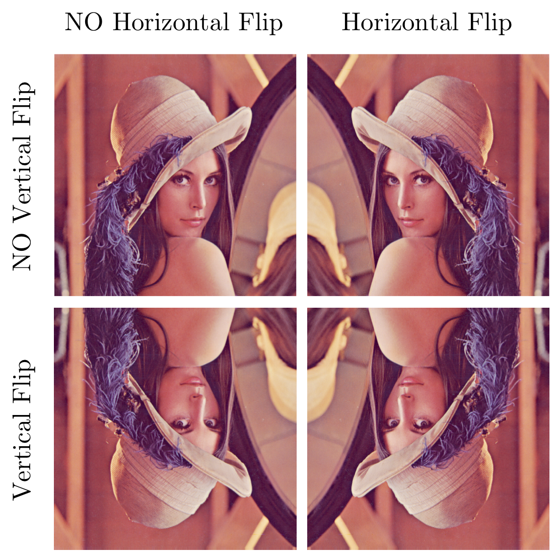
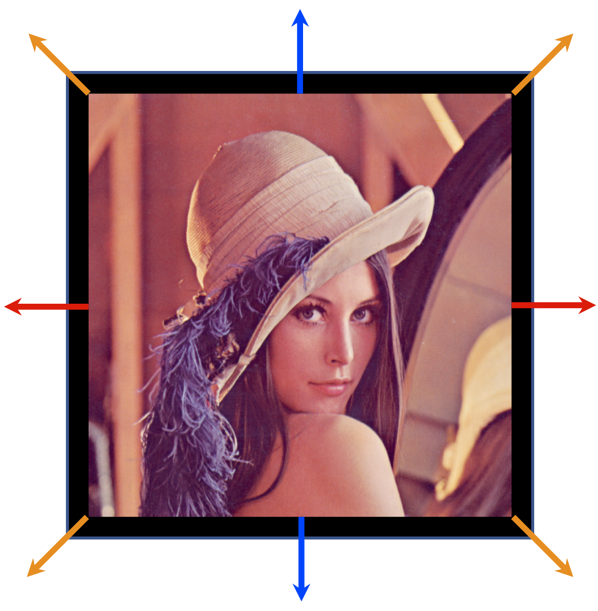
Left: Random Flipping; Right: Random Shifting.

Random Flipping is usually applied on each image during the training. The image can be translated into one of the four forms presented in the above left image randomly and independently. Note that for certain applications, one of vertical flipping or horizontal flipping might be disabled, e.g., for object segmentation in autonomous driving, it does not make sense to apply vertical flipping.

Random Shifting randomly shifts the image for some predefined distance along one of the 9 directions: left ( $\leftarrow$ ), right ( $\rightarrow$ ), up ( $\uparrow$ ), down ( $\downarrow$ ), up-left ( $\nwarrow$ ), up-right ( $\nearrow$ ), down-left ( $\swarrow$ ), down-right ( $\searrow$ ), and still ( $\cdot$ ) in the training phase (the above image at the right). This predefined distance is usually quantified in pixels.

Note that image augmentation is not applied in the testing phase because the goal is to reduce generalization error. There are other forms of image augmentation in practice, such as sample-wise standardization, whitening, rotating, scaling, shear transformation, contrast normalization.

Keras implementation

Keras implements many useful image geometric transformation and normalization methods. The description of the ImageDataGenerator is as follows:

keras.preprocessing.image.ImageDataGenerator(featurewise_center=False,
    samplewise_center=False,
    featurewise_std_normalization=False,
    samplewise_std_normalization=False,
    zca_whitening=False,
    zca_epsilon=1e-6,
    rotation_range=0.,
    width_shift_range=0.,
    height_shift_range=0.,
    shear_range=0.,
    zoom_range=0.,
    channel_shift_range=0.,
    fill_mode='nearest',
    cval=0.,
    horizontal_flip=False,
    vertical_flip=False,
    rescale=None,
    preprocessing_function=None,
    data_format=K.image_data_format())

This generator firstly takes the training features (e.g., $\mathbf{X}$ ) and then computes some statistics,

Here we show an example of using this ImageDataGenerator. This generator eliminates the feature-wise mean and normalizes the feature-wise standard deviation. Each image then randomly rotates for at most $20^{\circ}$ , shifts at most 20% both horizontally and vertically, and performs horizontal flip.

datagen = ImageDataGenerator(
    featurewise_center=True,
    featurewise_std_normalization=True,
    rotation_range=20,
    width_shift_range=0.2,
    height_shift_range=0.2,
    horizontal_flip=True)

# compute quantities required for featurewise normalization
# (std, mean, and principal components if ZCA whitening is applied)
datagen.fit(x_train)

# fits the model on batches with real-time data augmentation:
model.fit_generator(datagen.flow(x_train, y_train, batch_size=32),
                    steps_per_epoch=len(x_train) / 32, epochs=epochs)

Noted that this generator is implemented on CPU instead of GPU. Therefore, it takes a long time for preprocessing a huge dataset if you are not careful.

Exercises

Modify your ConvNet from last week so that now the network can be trained by using ImageDataGenerator and fit_generator APIs, see if there is any improvements in classification accuracy. Note that you should not apply certain augmentations that are applied on the training dataset on the testing dataset.
Run examples in the above contents, get familiar with OpenCV and scikit-image. (you don’t have to submit this part)