Welcome to the second session of Deep Learning in Raspberry Pi.
In this section, we are going to discuss some core concepts in Machine Learning (ML). We will dive into two historically very influential learning models: Linear Regression and Logistic Regression. We will also discuss Stochastic Gradient Descent (SGD) and its variants.
What is a “Learning Algorithm”?
A broadly adopted definition of the learning algorithm is given by Tom M. Mitchell in his classical book Machine Learning in 1997:
“A computer program is said to learn from
- experience with respect to
- some class of tasks and
- performance measure ,
if its performance at tasks in , as measured by , improves with experience ” (Mitchell, 1997)
Remark: This book is enjoyable to read and introduced many ML algorithms that were very popular back then. It reflects how researchers thought and did about ML in the 1980s and 1990s.
Many popular machine learning textbooks have in-depth discussions of this definition (Mitchell, 1997; Murphy, 2012; Goodfellow et al., 2016).
The task
The task is usually a specific problem that cannot be easily solved by conventional methods (e.g, array sorting problem can be easily solved by using quick sort). Here we provide some canonical examples of Machine Learning tasks:
-
Classification specifies which categories some input belongs to. ()
-
Regression predicts a numerical value given some input. ()
-
Transcription outputs a sequence of symbols, rather than a category code. (similar to classification, e.g., speech recognition, machine translation, image captioning)
-
Denoising predicts clean samples from corrupted samples . (estimate )
The performance measure
The performance measure is usually specific to the task (e.g. accuracy to classification). Unlike optimization, the learning algorithm is evaluated based on previously unseen data. We often have a set of validation data to conduct this evaluation. The design of a measure can be very subtle. The measure should be effective so that we can anticipate how well the learning algorithm would perform after deployment.
The experience
Experience is what learning algorithms are allowed to have during learning process. The experience is usually an dataset that is a collection of examples. Normally, we call this dataset as the training dataset. Here we give the structure of the training dataset to Unsupervised Learning and Supervised Learning algorithms.
-
Unsupervised Learning algorithms experience a dataset containing many features, learning useful structure of the dataset (estimate ).
-
Supervised Learning algorithms experience a dataset containing features, but each example is also associated with a label or target (estimate ).
Remark: In most real world cases, we would not have the access to the testing dataset and the validation dataset. In the absence of the validation dataset, we usually split 20% of the training dataset to be the validation dataset.
Hypothesis Function
Mathematically, this computer program with respect to the learning task can be defined as a hypothesis function that takes an input and transforms it to an output .
The function may be parameterized by a group of parameters . Note that includes both trainable and non-trainable parameters. All the DNN architectures discussed in this module can be formulated in this paradigm.
Strictly speaking, the hypothesis function defines a large family of functions that could be the solution to the task . At the end of training, the hypothesis function is expected to be parameterized by a set of optimal parameters that yields the highest performance according to the performance measure of the given task. Conventionally, we call the hypothesis function that equips the optimal parameters the trained model.
Cost Function
A cost function is selected according to the objective(s) of the hypothesis function in which it defines the constraints. The cost function is minimized during the training so that the hypothesis function can be optimized and exhibits the desired behaviors (e.g., classify images, predict houshold value, text-to-speech). The cost function reflects the performance measure directly or indirectly. In most cases, the performance of a learning algorithm gets higher when the cost function becomes lower.
When the cost function is differentiable (such as in DNNs presented in this module), a class of Gradient-Based Optimization algorithms can be applied to minimize the cost function . Thanks to specialized hardware such as GPUs and TPUs, these algorithms can be computed very efficiently.
Particularly, Gradient Descent (Cauchy, 1847) and its variants, such as
RMSprop (Tieleman & Hinton, 2012), Adagrad (Duchi et al., 2011), Adadelta
(Zeiler, 2012), Adam (Kingma & Ba, 2014) are surprisingly good at training
Deep Learning models and have dominated the development of training algorithms. Software libraries such as Theano (Theano Development Team, 2016)
and TensorFlow (Abadi et al., 2015) have automated the process of computing the gradient (the most difficult part of applying gradient descent) using
a symbolic computation graph. This automation enables the researchers to
design and train arbitrary learning models.
Remark: in this module, we use the term “cost function”, “objective function” and “loss function” interchangeably. Usually, the loss function is denoted as .
Ingredients to Solve a Machine Learning Task
Given a Machine Learning task, you need to have following ingredients for solving the task:
- A hypothesis function that maps the input features to outputs.
- A loss function that defines the objectives.
- A training algorithm that can optimize the loss function.
- A training dataset that contains a collection of training examples.
- A validation dataset that is used to evaluate the performance of the trained model.
- (Optional) A testing dataset that evaluates the performance of the trained model after deployment.
In this module, we will identify these ingredients while solving different tasks.
Linear Regression
Regression is a task of Supervised Learning. The goal is to take a input vector (a.k.a, features) and predict a target value . In this section, we will learn how to implement Linear Regression.
As the name suggests, Linear Regression has a hypothesis function that is a linear function. The goal is to find a linear relationship between the input features and the target value:
Note that is the -th sample in the dataset that has data points. The parameters consists of weights and a bias .
Suppose that the target value is a scalar (), we can easily define such a model in Keras:
x = Input((10,), name="input layer")  # the input feature has 10 values
y = Dense(1, name="linear layer")(x)  # implement linear function
model = Model(x, y)  # compile the hypothesis function
To find a linear relationship that has , we need to find a set of parameters from the parameter space where the optimized function generate least error as possible. Suppose we have a cost function that measures the error made by the hypothesis function, our goal can be formulated into:
For Linear Regression, one possible formulation of the cost function is Mean-Squared Error (MSE). This cost function measures the mean error caused by each data sample:
By minimizing this cost function via training algorithms such as Stochastic Gradient Descent (SGD), we hope that the trained model can perform well on unseen examples in the testing dataset.
Remark: there are other cost functions for regression tasks, such as Mean Absolute Error (MAE) and Root-Mean-Square-Error (RMSE). Interested readers are encouraged to find out what they are.
Remark: The math in this module chooses to use a column-vector based system, which means each vector is assumed to be a column vector. Many books and tutorials also apply this convention. However, in practice, most ndarray packages use the row-vector based system because the first dimension of a multi-dimensional array is for the row axis. For example,
A = np.array([1, 2, 3, 4, 5])
The array A is a row vector and has only the row axis. We assume that the readers know this fact and can modify the code accordingly.
Logistic Regression
In this section, we discuss the solution to another Supervised Learning task - Binary Classification. Instead of predicting continuous values (e.g., how many pairs of shoes you have), we wish to decide whether the input feature belongs to some category. In the case of Binary Classification, we have only two classes (e.g., to be or not to be, shoe or skirt). Logistic Regression is a simple learning algorithm that solves this kind of tasks.
Remark: Usually, we call a learning algorithm that solves binary classification a Binary Classifier.
Suppose our input feature is a -dimensional vector and the output class label (0 and 1 are abstract labels, we can associate meanings for these labels, such as 0 is shoe and 1 is skirt). The Logistic Regression constructs a hypothesis function that assigns the probability that belongs to the class . Specifically, the Logistic Regression uses the “logistic function”. The hypothesis function is then described as follows:
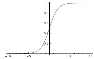
The logistic function.
Here, we use the symbol to represent the logistic function. Furthermore, is often called the “sigmoid” function as well. The logistic function has a nice property where it can map the input into the range so that we can interpret the output of this function as probability:
Now, we need to design a cost function. The desired function for measuring the quality of the prediction is binary cross-entropy:
Intuitively, when the model makes a correct decision (suppose the true label is 1), then the is also high, this generates a lower cost when the model makes a wrong decision and the is low. From the information theoretic point of view, the cross-entropy between a “true” distribution and an estimated distribution measures the “similarity” between two distributions. Ideally, when the number of sample and cost function , we cannot distinguish the estimation distribution from the “true” distribution.
Our learning algorithm is expected to find a best set of parameters that minimizes the cost function :
Note that there is a close tie between the Logistic Regression and the Linear Regression. The Logistic Regression is nothing more than adding a non-linear function on top of the linear function. Here is an example of logistic regression in Keras:
x = Input((10,), name="input_layer")
y = Dense(1, name="linear layer")(x)
y = Activation("sigmoid")(y)
model = Model(x, y)
Remark: we will revisit the logistic function in Session 3 when we introduce the first neural network model: Multi-layer Perceptron.
Logistic Regression is designed to solve Binary Classification tasks. The above formulation can be generalized to solve Multi-class Classification tasks. The following equation defines the hypothesis function for the extension of the Logistic Regression - Softmax Regression:
where is the -th column of a weight matrix and is the corresponding bias value.
The cost function is defined with categorical cross-entropy function:
is the “indicator function” so that and otherwise.
Note that we do not explain this loss function here in detail. The Deep Learning book has a very nice explanation of Softmax function in Section 6.2.2.3.
The optimization algorithm finds a set of parameters that minimizes the cost function:
Here is a Keras example
x = Input((10,), name="input_layer")
y = Dense(5, name="linear layer")(x)  # suppose there are 5 classes
y = Activation("softmax")(y)
model = Model(x, y)
Remark: Although we do not explain the Softmax Regression in details, in fact, the function is widely used by many modern deep learning systems for solving fundamental problems such as classification, and complicated tasks such as neural machine translation.
Stochastic Gradient Descent and its Variants
Previous sections define the learning models for Regression and Binary Classification tasks. We now need a training algorithm that minimizes the cost function described in the above sections. In this section, we introduce the most famous set of Gradient-based Optimization algorithms – Stochastic Gradient Descent (SGD) and its variants.
Almost all modern Deep Learning models are trained by the variants of SGD. In some particular cases, there are deep learning models that are trained with second-order gradient-based methods (e.g., Hessian optimization).
To describe SGD, we first need to understand its parent method - Gradient Descent. The idea of Gradient Descent is very simple: Suppose that we need to iteratively refine the parameters so that we can minimize the cost function . The best direction that we should take follows the direction of the steepest descent. This direction can be computed by evaluating the gradient of the loss function. The core idea of the Gradient Descent can be described as follows:
where is the updated parameters, computes the updating directions and the learning rate controls the step size that is taken at the current update. Note that the cost function is a data-driven function where the training data is used to calculate the update. We sometimes call the above formulation as “vanilla” Gradient Descent.
The learning rate is arguably the most important hyperparameter in training Deep Learning models. If you set the learning rate too large, then the step update may overshoot and leads to worse performance. On the other hand, if you set the learning rate too small, then the training process may take a longer time to complete.
Remark: Hyperparameters are settings that control the behavior of the learning algorithm. Usually we choose them empirically.
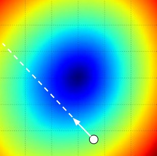
Visualizing the effect of step size. The white arrow points to the steepest direction. Image credit: CS231n
In most cases, it is not feasible to use Gradient Descent because the training dataset is too large to evaluate. Instead, a common practice is to compute the gradient over batches of training examples. The parameters are updated after evaluating each batch of data. The reason this technique works is that the samples in the training dataset are correlated. However, this technique also introduces stochasticity into the parameter update. Hence this type of training algorithm is called Stochastic Gradient Descent (SGD). And because we most commonly use mini-batches, sometimes people also refer this training algorithm as mini-batch SGD.
Gradient Descent is guaranteed to converge to the global minimum if the cost function is a convex function. In most cases, the cost functions are non-convex functions. In these cases, Gradient Descent can only find the local-minima.
Momentum SGD
The vanilla SGD can lead easily to traps around a local minimum point. For example, in such a case, all the directions around the local region seem steep. The parameters then oscillate around this local region during training. To get out of the local minima, we can use a variant of the vanilla SGD - Momentum SGD. The formulation is as follows:
The basic idea is that if we allow the gradient update to accumulate, at some point, the energy of the update is powerful enough to jump out from the local minima. With momentum, we gain faster convergence and less oscillatory behavior. Empirically, the momentum parameter is set to 0.9 or 0.99.
Remark: .
Adaptive SGD
Choosing the learning rate for SGD is mainly empirical. Therefore, we will have to perform a manual search from a list of possible learning rates. This process is usually costly and time-consuming. In recent years, researchers developed a set of SGD variants that adjust the learning rate automatically.
The notable examples are RMSprop (Tieleman & Hinton, 2012), Adagrad (Duchi et al., 2011), Adadelta (Zeiler, 2012), Adam (Kingma & Ba, 2014).
Note that the motivation of having these different variants is not entirely because of the dissatisfaction of the SGD and brute-force search for the learning rate. For example, RMSprop is proposed to deal with the vanishing gradient problem where some very deep networks cannot be trained with standard SGD.
Empirically, one should use Adam optimizer as a starting point.
Comparing different gradient optimization methods. Left: SGD optimization on saddle point. Right: SGD optimization on loss surface contours. Image credit: Alec Radford
Learning Rate Scheduling
The above sections discuss the methods that have a fixed initial learning rate. The learning rate is either static or adjusted by the training algorithm itself. Recent research suggests that instead of using these optimizers, it is better to schedule the learning rate throughout the training. Normally, this involves even more expensive parameter searching because the researcher has to predefine the “schedule” of the use of learning rate at the different stages of training.
Fortunately, over the years, there are some empirical training schedules that work well across the tasks. We do not discuss this in detail since this is out of scope of this module. However, we do encourage readers to find some recent papers in large scale image recognition and natural language processing papers where they employ such training schedules.
Remark: SGD and its variants represent the most popular group of training algorithms. However, there are other optimization algorithms available and extensively studied by Machine Learning researchers, such as energy based models, evolutionary algorithms, genetic algorithms, Bayesian optimization.
Remark: Sebastian Ruder surveyed almost all popular variants of SGDs in a blog post.
Training model in Keras
After you have defined a model by using the Model class (see above model examples for linear regression, logistic regression, and softmax regression), you will need to compile the model with some loss function and an optimizer. In Keras, we can use the compile API:
model.compile(loss="mean_squared_error",
              optimizer="sgd",
              metrics=["mse"])
The above example compiled a Linear Regression model that uses MSE as the loss function and the default SGD as the optimizer. The performance measure here is called metrics. You can have different metrics for evaluating the performance of the model. We also use MSE as the metric for evaluation. If you have a classification task, you can change the loss and metrics to other options. You can find more about losses and metrics in the Keras documentation.
You can then train the model with the data once the model is compiled. Here is an example:
model.fit(
    x=train_X, y=train_y,
    batch_size=64, epochs=10,
    validation_data=(test_X, test_y))
The API fit essentially takes your training data and schedule them into a training routine. First, you need to specify your training inputs x and training target y. And then you will need to define the mini-batch size and number of epochs. The fit API will run for number of epochs times and then at each step of a epoch, the function will fetch a batch of training examples (in this case, 64) and then use them to compute the gradient update. The parameters are updated after the
gradient is computed. Finally, we can supply a set of validation data (in this case, (test_X, test_y). After each training epoch, Keras evaluates the model’s performance using the validation data.
Remark: the fit function essentially implements mini-batch SGD and its variants. A training step is performed when one batch of training examples are used to update the parameters. Once all batches of training examples are used, the training finishes one training epoch.
Remark: The fit function is not the only way you can do training, when you are dealing with larger dataset or have some preprocessing for the data, you can use fit_generator to schedule your training.
Generalization
Typically, we expect that the trained model can be used to predict new, unseen samples. This ability to perform well on previously unobserved data is called generalization. With a performance measure , we can compute the error that is made over the training dataset. This error is called training error. We can also compute the testing error with the validation dataset or the testing dataset if available. This testing error quantifies the level of generalization of a certain model. Our goal is to minimize this testing error and improve the generalization.
Because we can only observe the training dataset during training, our trained model may suffer from either overfitting or underfitting. Overfitting occurs when the gap between the training error and testing error is too large. Underfitting occurs when the model is not able to obtain a sufficiently low error value on the training dataset.
We can control whether a model is more likely to overfit or underfit by altering its capacity. Informally, a model’s capacity is its ability to fit a wide variety of functions. Ideally, we want to find a model that has the optimal capacity where the model generates the smallest gap between the training error and the testing error.
Usually, Deep Learning models have tremendous capacity. These models almost always overfit the dataset given enough training time. Strangely, these models also exhibit strong generalization over testing dataset with the help of different training techniques. One straightforward technique is Early Stopping. The Early Stopping technique stops the training when the model starts to overfit.
No Free Lunch Theorem and Curse of Dimensionality
No Free Lunch Theorem
To solve one particular task, we can choose from many different models and learning algorithms. Empirically, we can evaluate the performance of these models and algorithms using the validation dataset. However, there is no universally best model – this is the famous no free lunch theorem (Wolpert, 1996). The reasons for this is that different models make different assumptions. These assumptions may work well in one domain and work poorly in another domain. As a consequence, rather than focusing on developing the universal model, we seek the solution that performs well in a practical scenario for some relevant domains or distributions.
Curse of Dimensionality
Many machine learning problems become exceedingly difficult when the number of dimensions in the data is high. The phenomenon is known as the curse of dimensionality. Of particular concern is that the number of possible distinct configurations of the variables of interest increases exponentially as the dimensionality increases.
Remark: For elaborated description of these two challenges, please refer to the Chapter 5 of the Deep Learning book and Chapter 1 of the book Machine Learning: A probabilistic perspective.
Exercises
In this exercise, you will need to implement Logistic Regression to distinguish two classes from the Fashion-MNIST dataset.
We provide some useful functions for accessing the Fashion-MNIST datasets in pnslib, please first clone and install the pnslib by:
$ git clone https://github.com/PnS2018/pnslib
$ cd pnslib
$ python setup.py develop  # add sudo in front if there is a permission error.
Note that we are going to use pnslib package for both exercises and projects in future. You will need to update the package for the latest changes.
$ cd pnslib
$ git pull origin master
-
We provide a template script that has the barebone structure of implementing Logistic Regression in Keras. You will need to complete the script and get it running. You are expected to define a Logistic Regression model, compile the model with binary cross-entropy loss and a optimizer, and train the model. If you can successfully train the model, try to change the choice of optimizer, what do you observe?
-
In this exercise, you will implement the Logistic Regression from scratch. We provide a template script that contains necessary setup code, you need to complete the code and run. You are expected to write a training loop that can loop over the data for some number of epochs.